43 how to customize data labels in excel
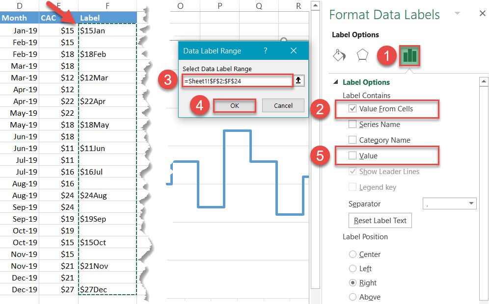
How to Customize Your Excel Pivot Chart Data Labels - dummies To add data labels, just select the command that corresponds to the location you want. To remove the labels, select the None command. If you want to specify what Excel should use for the data label, choose the More Data Labels Options command from the Data Labels menu. Excel displays the Format Data Labels pane. How to Use Cell Values for Excel Chart Labels Select the chart, choose the "Chart Elements" option, click the "Data Labels" arrow, and then "More Options.". Uncheck the "Value" box and check the "Value From Cells" box. Select cells C2:C6 to use for the data label range and then click the "OK" button. The values from these cells are now used for the chart data labels.
Add / Move Data Labels in Charts - Excel & Google Sheets Click on the graph Select + Sign in the top right of the graph Check Data Labels Change Position of Data Labels Click on the arrow next to Data Labels to change the position of where the labels are in relation to the bar chart Final Graph with Data Labels

How to customize data labels in excel
How to Create Mailing Labels in Excel | Excelchat In this tutorial, we will learn how to use a mail merge in making labels from Excel data, set up a Word document, create custom labels and print labels easily. Figure 1 - How to Create Mailing Labels in Excel. Step 1 - Prepare Address list for making labels in Excel. First, we will enter the headings for our list in the manner as seen below. How to add data labels from different column in an Excel chart? Right click the data series, and select Format Data Labels from the context menu. 3. In the Format Data Labels pane, under Label Options tab, check the Value From Cells option, select the specified column in the popping out dialog, and click the OK button. Now the cell values are added before original data labels in bulk. 4. Custom data labels in a chart - Get Digital Help Press with right mouse button on on any data series displayed in the chart. Press with mouse on "Add Data Labels". Press with mouse on Add Data Labels". Double press with left mouse button on any data label to expand the "Format Data Series" pane. Enable checkbox "Value from cells".
How to customize data labels in excel. How to Change Excel Chart Data Labels to Custom Values? You can change data labels and point them to different cells using this little trick. First add data labels to the chart (Layout Ribbon > Data Labels) Define the new data label values in a bunch of cells, like this: Now, click on any data label. This will select "all" data labels. Now click once again. Edit titles or data labels in a chart - support.microsoft.com The first click selects the data labels for the whole data series, and the second click selects the individual data label. Right-click the data label, and then click Format Data Label or Format Data Labels. Click Label Options if it's not selected, and then select the Reset Label Text check box. Top of Page How to Create Labels in Word from an Excel Spreadsheet Enter the Data for Your Labels in an Excel Spreadsheet 2. Configure Labels in Word 3. Bring the Excel Data Into the Word Document 4. Add Labels from Excel to a Word Document 5. Create Labels From Excel in a Word Document 6. Save Word Labels Created from Excel as PDF 7. Print Word Labels Created From Excel 1. How to I rotate data labels on a column chart so that they are ... To change the text direction, first of all, please double click on the data label and make sure the data are selected (with a box surrounded like following image). Then on your right panel, the Format Data Labels panel should be opened. Go to Text Options > Text Box > Text direction > Rotate
Using the CONCAT function to create custom data labels for an Excel ... Use the chart skittle (the "+" sign to the right of the chart) to select Data Labels and select More Options to display the Data Labels task pane. Check the Value From Cells checkbox and select the cells containing the custom labels, cells C5 to C16 in this example. It is important to select the entire range because the label can move based ... Excel tutorial: How to use data labels Generally, the easiest way to show data labels to use the chart elements menu. When you check the box, you'll see data labels appear in the chart. If you have more than one data series, you can select a series first, then turn on data labels for that series only. You can even select a single bar, and show just one data label. how to add data labels into Excel graphs - storytelling with data Right-click on a point and choose Add Data Label. You can choose any point to add a label—I'm strategically choosing the endpoint because that's where a label would best align with my design. Excel defaults to labeling the numeric value, as shown below. Now let's adjust the formatting. How to Create Address Labels from Excel on PC or Mac menu, select All Apps, open Microsoft Office, then click Microsoft Excel. If you have a Mac, open the Launchpad, then click Microsoft Excel. It may be in a folder called Microsoft Office. 2. Enter field names for each column on the first row. The first row in the sheet must contain header for each type of data.
Custom Chart Data Labels In Excel With Formulas Follow the steps below to create the custom data labels. Select the chart label you want to change. In the formula-bar hit = (equals), select the cell reference containing your chart label's data. In this case, the first label is in cell E2. Finally, repeat for all your chart laebls. How do I create a one variable data table in Excel? In Excel 2016 for Mac: Click Data > What-if Analysis > Data Table. In Excel for Mac 2011: On the Data tab, under Analysis, click What-If, and then click Data Table. In the Row input cell box, enter the reference to the input cell for the input values in the row. How to add or move data labels in Excel chart? - ExtendOffice 2. Then click the Chart Elements, and check Data Labels, then you can click the arrow to choose an option about the data labels in the sub menu. See screenshot: In Excel 2010 or 2007. 1. click on the chart to show the Layout tab in the Chart Tools group. See screenshot: 2. Then click Data Labels, and select one type of data labels as you need ... Add Custom Labels to x-y Scatter plot in Excel Step 1: Select the Data, INSERT -> Recommended Charts -> Scatter chart (3 rd chart will be scatter chart) Let the plotted scatter chart be. Step 2: Click the + symbol and add data labels by clicking it as shown below. Step 3: Now we need to add the flavor names to the label. Now right click on the label and click format data labels.

Australia - Geographic State Heat Map - Excel Template - INDZARA
How to add and customize chart data labels - Get Digital Help Double press with left mouse button on with left mouse button on a data label series to open the settings pane. Go to tab "Fill & Line" and expand "Fill" settings, see image to the right. These settings allow you to change the background to a solid fill, gradient fill, picture or texture fill, pattern fill, or Automatic. Border
Customize Polar Axes - MATLAB & Simulink
How to create Custom Data Labels in Excel Charts Two ways to do it. Click on the Plus sign next to the chart and choose the Data Labels option. We do NOT want the data to be shown. To customize it, click on the arrow next to Data Labels and choose More Options … Unselect the Value option and select the Value from Cells option. Choose the third column (without the heading) as the range.
Enable or Disable Excel Data Labels at the click of a button - How To - PakAccountants.com
How to Create Mailing Labels in Word from an Excel List Step Two: Set Up Labels in Word. Open up a blank Word document. Next, head over to the "Mailings" tab and select "Start Mail Merge.". In the drop-down menu that appears, select "Labels.". The "Label Options" window will appear. Here, you can select your label brand and product number. Once finished, click "OK.".
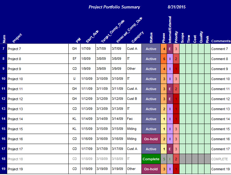
Project Status Analysis Workbook
Change the format of data labels in a chart To get there, after adding your data labels, select the data label to format, and then click Chart Elements > Data Labels > More Options. To go to the appropriate area, click one of the four icons ( Fill & Line, Effects, Size & Properties ( Layout & Properties in Outlook or Word), or Label Options) shown here.
How to Create a Step Chart in Excel - Automate Excel
Add a DATA LABEL to ONE POINT on a chart in Excel All the data points will be highlighted. Click again on the single point that you want to add a data label to. Right-click and select ' Add data label '. This is the key step! Right-click again on the data point itself (not the label) and select ' Format data label '. You can now configure the label as required — select the content of ...

How to Create Multi-Category Chart in Excel - Excel Board
How to create label cards in Excel - Ablebits You can select any other range or enter it using your keyboard. Click the Expand selection icon to have the entire table highlighted automatically. Use the Select range option to collapse the dialog window and choose the range you need: If the top row in the selected table is a header, tick off this option. Tip.
How to Import Excel Data into a Label File in Text Labels | Brady Support
Custom Data Labels with Colors and Symbols in Excel Charts - [How To] To apply custom format on data labels inside charts via custom number formatting, the data labels must be based on values. You have several options like series name, value from cells, category name. But it has to be values otherwise colors won't appear. Symbols issue is quite beyond me.

Excel charts: add title, customize chart axis, legend and data labels
How to Print Labels From Excel - Lifewire Choose Start Mail Merge > Labels . Choose the brand in the Label Vendors box and then choose the product number, which is listed on the label package. You can also select New Label if you want to enter custom label dimensions. Click OK when you are ready to proceed. Connect the Worksheet to the Labels

» Excel Charts: Creating Custom Data Labels
Apply Custom Data Labels to Charted Points - Peltier Tech Double click on the label to highlight the text of the label, or just click once to insert the cursor into the existing text. Type the text you want to display in the label, and press the Enter key. Repeat for all of your custom data labels. This could get tedious, and you run the risk of typing the wrong text for the wrong label (I initially ...
Add or remove data labels in a chart - Office Support
How Do I Create Avery Labels From Excel? - Ink Saver Create the Spreadsheet: Open your MS Excel and start creating the spreadsheet in question. Fill out all the data you need to be labeled. Once done, save the document to a directory you can remember as we will use it later in the procedure. 2.
Free Assets Business database templates for Organizer Advantage users.
Custom data labels in a chart - Get Digital Help Press with right mouse button on on any data series displayed in the chart. Press with mouse on "Add Data Labels". Press with mouse on Add Data Labels". Double press with left mouse button on any data label to expand the "Format Data Series" pane. Enable checkbox "Value from cells".
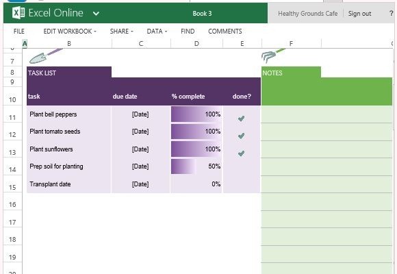
Free Garden Planner Excel Template
How to add data labels from different column in an Excel chart? Right click the data series, and select Format Data Labels from the context menu. 3. In the Format Data Labels pane, under Label Options tab, check the Value From Cells option, select the specified column in the popping out dialog, and click the OK button. Now the cell values are added before original data labels in bulk. 4.
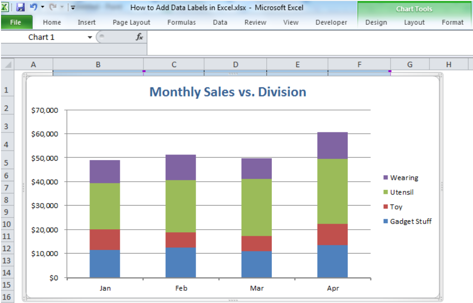
How to Add Data Labels in Excel - Excelchat | Excelchat
How to Create Mailing Labels in Excel | Excelchat In this tutorial, we will learn how to use a mail merge in making labels from Excel data, set up a Word document, create custom labels and print labels easily. Figure 1 - How to Create Mailing Labels in Excel. Step 1 - Prepare Address list for making labels in Excel. First, we will enter the headings for our list in the manner as seen below.

Charting in Excel - Adding Data Labels - YouTube

How to Add Data Labels in Excel - Excelchat | Excelchat
Create a Histogram Graph in Excel
Post a Comment for "43 how to customize data labels in excel"